Two-body decaying dark matter

Description

TBDemu is an emulator implementing a nonlinear response of two-body decays within the dark matter. The phenomenology of two-body decaying dark matter (2bDDM) is based on two parameters: the decay rate \(\Gamma\) (in 1/Gyr) and the magnitude of velocity kicks obtained by decay products \(v_k\) (in km/s). Additionally, one can assume only a fraction of decaying dark matter \(f\) in the total dark matter abundance: \(f=\Omega_{\rm m, decaying}/\Omega_{\rm m, total}\). The TBDemu emulator is built on gravity-only \(N\)-body simulations run by Pkdgrav3 code [1]. The emulator predicts

\[\mathcal{S}^{\Gamma,v_k,f}_{\rm DDM}(k,z) = P^{\Gamma,v_k,f}_{\rm DDM}(k,z)/P_{\Lambda \rm CDM}(k,z),\]

thus a ratio of nonlinear matter power spectrum in the scenario including dark matter decays and (nonlinear) \(\Lambda \rm CDM\) matter power spectrum. For more details, see Ref. [2]. The emulator was trained using Sinusoidal representation networks (SIRENs) [3].

Quickstart

import numpy as np
import DMemu
import matplotlib.pyplot as plt

# load emulator
emul = DMemu.TBDemu()

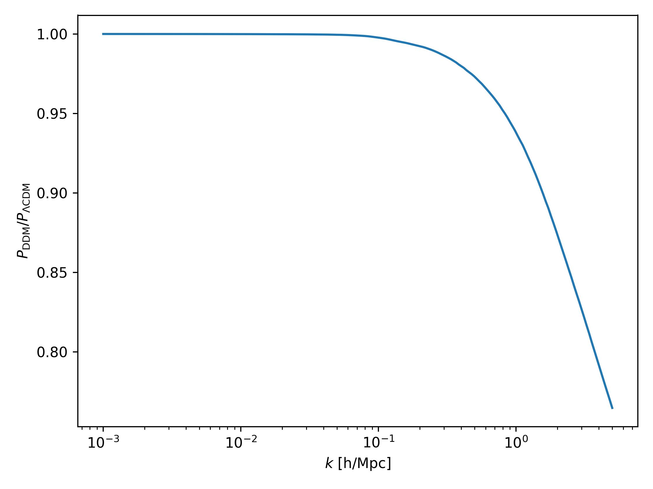
# predict suppressions between kmin and kmax for a single redshift
kmin = 1e-3 # in h/Mpc
kmax = 5 # in h/Mpc
ks = np.logspace(np.log10(kmin),np.log10(kmax),200) # scales
zs = 0.0 # redshift
velocity_kick = 500 # in km/s
gamma_decay = 1/50 # in 1/Gyr
fraction = 1.0

pks = emul.predict(ks,zs,fraction,velocity_kick,gamma_decay)

# plot
plt.semilogx(ks,pks)
plt.xlabel(r'$k$ [h/Mpc]')
plt.ylabel(r'$P_{\rm DDM}/P_{\Lambda \rm CDM}$')
plt.tight_layout()
plt.show()

Parameter space

• decay rate: \(\Gamma \in [0,1/13.5]\) Gyr \(^{-1}\)

• velocity kick magnitude: \(v_k \in [0,5000]\) km/s

• fraction of 2bDDM: \(f \in [0,1]\)

• scales: \(k < 6\) h/Mpc

• redshifts: \(z < 2.35\)

Input format of \(k\) and \(z\)

1. Single value of \(k\) and \(z\):

   k = 0.10 # in h/Mpc
   z = 0.0
   pks = emul.predict(k,z,fraction,velocity_kick,gamma_decay)
   

   Provides a single suppression value.

2. Single value of \(z\) for multiple scales \(k\):

   k = np.logspace(-2,0,10) # in h/Mpc
   z = 0.0
   pks = emul.predict(k,z,fraction,velocity_kick,gamma_decay)
   

   Provides a list of suppressions at desired scales for a single redshift \(z\).

3. Single value of \(k\) for multiple redshifts \(z\):

   k = 0.10 # in h/Mpc
   z = np.array([0.0,1.0,2.0])
   pks = emul.predict(k,z,fraction,velocity_kick,gamma_decay)
   

   Provides a list of suppressions at a given scale for all redshift values \(z\).

4. Multiple scales \(k\) for multiple redshifts \(z\):

   k = np.array([0.1,0.5,1.0]) # in h/Mpc
   z = np.array([0.0,1.0,2.0])
   pks = emul.predict(k,z,fraction,velocity_kick,gamma_decay)
   

The above code provides three suppression values, first for \(k=0.1\) and \(z=0.0\), second for \(k=0.5\) and \(z=1.0\) and last for \(k=1.0\) and \(z=2.0\). The code checks that the lengths of both array are equal.

Extrapolation

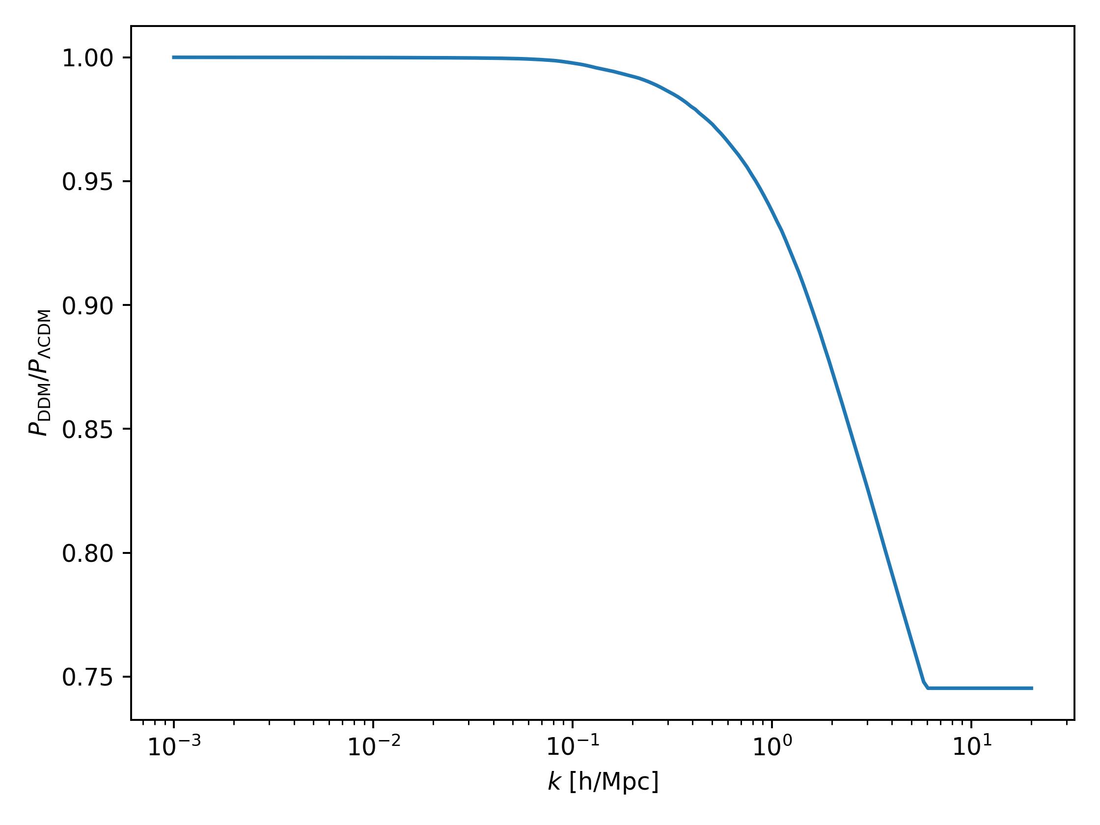
Extrapolation for \(\Gamma\), \(v_k\), \(f\) and \(z\) is not allowed as the trained architecture cannot reliably predict outside the training domain. Extrapolation for \(k>6\) h/Mpc is done by adding a constant suppression continuously attached to the one provided by an emulator, see the figure below. However, one can ask for redshifts higher than 2.35 by setting allow_z_extrapolation=True in TBD.predict(...) function.

References

[1]

Bucko, J., Giri, S. K., Hervas Peters, F., & Schneider, A. Probing the two-body decaying dark matter scenario with weak lensing and the cosmic microwave background. A&A 683 A152 (2024). https://doi.org/10.1051/0004-6361/202347844

[2]

Potter, D., Stadel, J. & Teyssier, R. PKDGRAV3: beyond trillion particle cosmological simulations for the next era of galaxy surveys. Comput. Astrophys. 4, 2 (2017). https://doi.org/10.1186/s40668-017-0021-1

[3]

Sitzmann, V., Martel, J. N. P., Bergman, A. W., Lindell, D. B., & Wetzstein, G. (2020). Implicit Neural Representations with Periodic Activation Functions. Proc. NeurIPS.