One-body decaying dark matter
Description
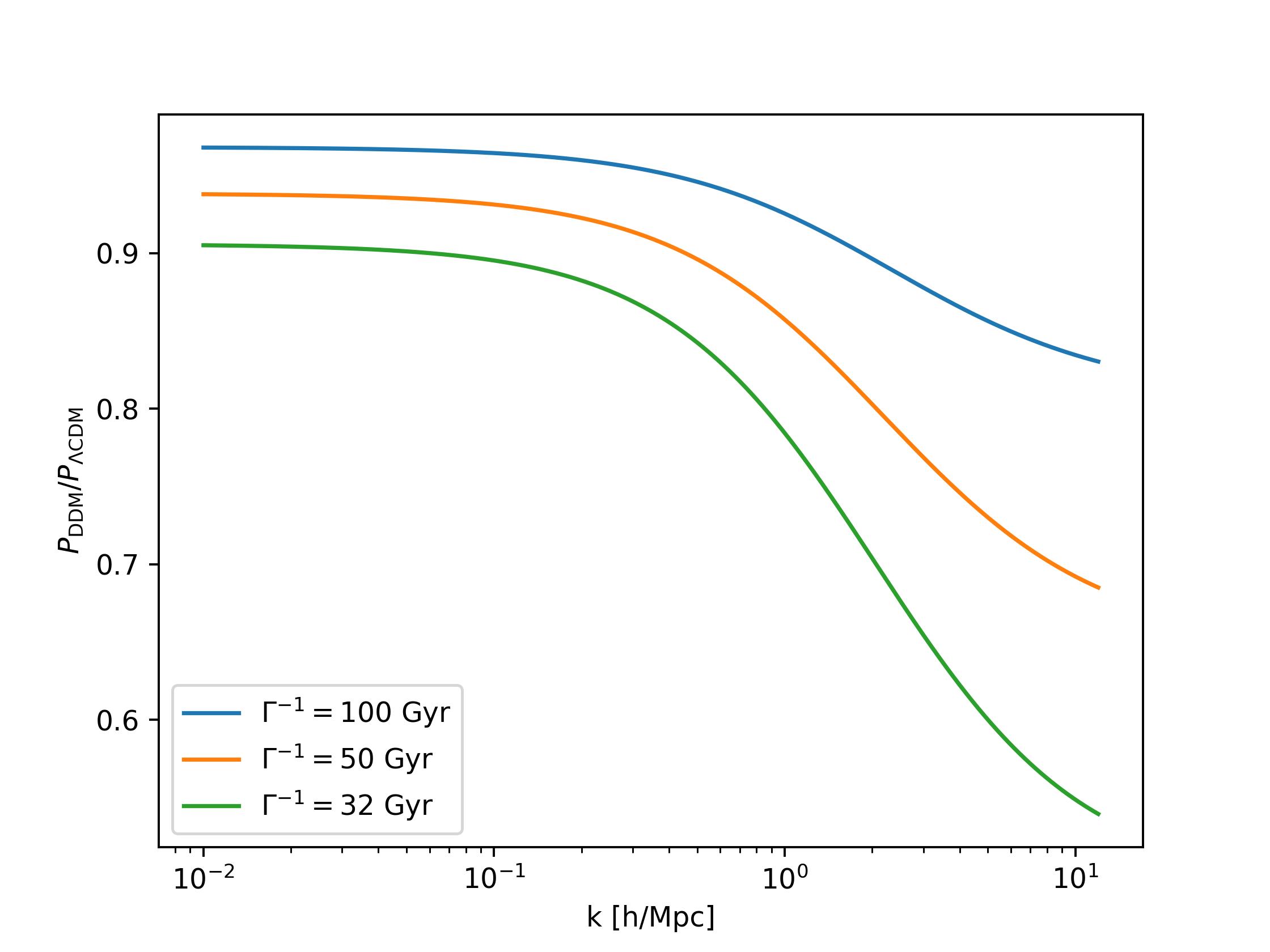
OBDemu is an emulator implementing a fitting formulae predicting nonlinear matter power spectra in the presence of one-body decays within the dark sector. The decays are described by a decay rate \(\Gamma\) (in 1/Gyr) and a fraction of decaying dark matter \(f\) inside the total dark matter abundance: \(f=\Omega_{\rm m, decaying}/\Omega_{\rm m, total}\). The OBDemu emulator is built based on gravity-only \(N\)-body simulations run by Pkdgrav3 code [1]. The emulator predicts
thus a ratio of nonlinear matter power spectrum in the scenario including dark matter decays and (nonlinear) \(\Lambda \rm CDM\) matter power spectrum. For more details and the specific shape of fitting functions, see Ref. [2].
Quickstart
import numpy as np
import DMemu
import matplotlib.pyplot as plt

# load emulator
emul = DMemu.OBDemu()

# predict suppressions between kmin and kmax for a single redshift
kmin = 1e-2 # h/Mpc
kmax = 12 # h/Mpc
ks = np.logspace(np.log10(kmin),np.log10(kmax),1000)
zs = 0.0
Omega_b = 0.049
Omega_m = 0.315
h = 0.67

for gamma_decay in [1/100,1/50,1/32]:
    f = 1.0
    pks = emul.predict(ks,zs,gamma_decay,f,Omega_b,Omega_m,h)
    # plot
    plt.semilogx(ks,pks,label = r'$\Gamma^{-1} = %.0f$ Gyr'%(1.0/gamma_decay))

plt.legend()
plt.xlabel('k [h/Mpc]')
plt.ylabel(r'$P_{\rm DDM}/P_{\Lambda \rm CDM}$')
plt.tight_layout()
plt.show()
Parameter space
The analytical fitting formulae can be easily and naturally extrapolated, however, their precision have been tested in the following domain:
decay rate: \(\Gamma \in [0,1/31.6]\) Gyr \(^{-1}\)
fraction of 1bDDM: \(f \in [0,1]\)
scales: \(k < 10\) 1/Mpc
redshifts: \(z < 2.35\)
baryonic abundance \(\omega_b \in [0.019,0.026]\)
matter abundance \(\omega_m \in [0.09,0.28]\)
hubble parameter \(h \in [0.6,0.8]\)
Input format of \(k\) and \(z\)
Single value of \(k\) and \(z\):
k = 0.10 # in h/Mpc
z = 0.0
pks = emul.predict(k,z,gamma_decay,fraction)
Provides a single suppression value.
Single value of \(z\) for multiple scales \(k\):
k = np.logspace(-2,0,10) # in h/Mpc
z = 0.0
pks = emul.predict(k,z,gamma_decay,fraction)
Provides a list of suppressions at desired scales for a single redshift \(z\).
Single value of \(k\) for multiple redshifts \(z\):
k = 0.10 # in h/Mpc
z = np.array([0.0,1.0,2.0])
pks = emul.predict(k,z,gamma_decay,fraction)
Provides a list of suppressions at a given scale for all redshift values \(z\).
Multiple scales \(k\) for multiple redshifts \(z\):
k = np.array([0.1,0.5,1.0]) # in h/Mpc
z = np.array([0.0,1.0,2.0])
pks = emul.predict(k,z,gamma_decay,fraction)
The above code provides three suppression values, first for \(k=0.1\) and \(z=0.0\), second for \(k=0.5\) and \(z=1.0\) and last for \(k=1.0\) and \(z=2.0\). The code checks that the lengths of both array are equal.
Extrapolation
Extrapolation for \(\Gamma\), \(f\) and \(z\) is naturally provided by the fitting formulae but the precision is not guaranteed. A warning will show up as soon as the input value falls outside of the emulator’s domain.